Yesterday I read a nice post called “doubly dual shuffles”, which¹ pointed out something about the classic algorithm for shuffling an array (i.e. sampling a uniformly random permutation of it).

It’s a concise and (his word!) “pearlescent” post and you should read it, but in short, even modulo a simple and uninteresting “mirroring” (where you can move left-to-right or right-to-left), there are actually two distinct algorithms:

• in one of them, at each step you “sample” from the “rest” of the array,
• in the other one, at each step you “permute” the elements seen so far.

This was really surprising to me, because I must have coded a shuffle like this dozens of times, but I had never thought of the latter variant. And the difference between the two shows up even more starkly when we try to analyze the corresponding algorithms for generating random cyclic permutations, as we’ll see below.

To make this clearer, I worked with Claude (transcript) for a while to have it generate the visualizations below, all for shuffling an array of 10 elements, initially containing 0, 1, …, 9. The visualizations all go from left to right by default, but each of them has a toggle button to go the other way.

The first one is the “sampling” shuffle, which is the way I’ve always encountered or written it. (For what it’s worth I’ve always written it going left-to-right, but actually Knuth in The Art of Computer Programming follows Richard Durstenfeld and gives it going right-to-left):

The algorithm is as follows:

• Initially none of the elements are “done” (green).
• At each step, we pick the next not-done element, and swap it with a random element of the part of the array starting at this element (possibly itself), and mark it “done”.

The invariant at each step is that the “done” elements form a uniformly random sample from all ways of arranging those many elements from the array. (That is, after $k$ steps, each of the $\displaystyle k!{n \choose k}$ possibilities is equally likely, until with $k=n$ we have a uniformly random permutation of the initial array.)

The alternative, which is a minor tweak to the random sampling but completely different in how it works, is as below:

Here, the algorithm is:

• Initially, none of the elements is “done”.
• At each step, we pick the next not-done element, and swap it with a random element of the part of the array ending at this element (possibly itself), and mark it “done”.

The invariant in this case is that the “done” elements form a uniformly random permutation of the part of the array they cover: the set of elements is the same as initially, but their ordering is uniformly random. (That is, after $k$ steps each of the $k!$ permutations of those $k$ elements is equally likely, until with $k=n$ we have uniformly sampled from all $n!$ permutations of the original array.)

As mentioned above, I had never thought of this… although I came close to noticing it, in the context of generating random cyclic permutations:

Cyclic permutations

The post also mentions:

There’s a classic off-by-one mistake that turns a shuffle into Sattolo’s algorithm for cyclic permutations. It happens when the random bounds are too narrow, so that is never equal to this, and an element can never land in the same place that it started. This change has the same effect on both kinds of shuffle.

and this Sattolo’s algorithm was something I had encountered only recently. (I’m old enough that anything less than a decade ago counts as “recently”.) Specifically, a minor tweak to the algorithm, which one might even accidentally (and mistakenly) do as an “optimization”—namely, not allowing an element to swap with itself—leads to an algorithm that instead randomly samples from permutations containing only one cycle:

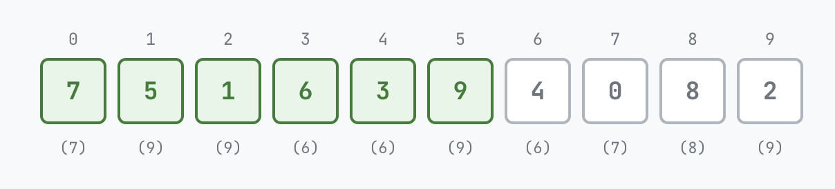
This visualization requires more explanation and the invariant is also harder to state. The number in parenthesis below each element shows the largest (or if going right-to-left, the smallest) element in the cycle it is part of.

This algorithm is known as Sattolo’s algorithm after Sandra Sattolo who published it in 1986. Its correctness is not as trivial to see! When I encountered the post by Dan Luu where I first heard about this algorithm, I tried reading the proof quickly, dismissed it as probably harder than it needed to be, skimmed through a reference titled Overview of Sattolo’s algorithm linked from Wikipedia, and went ahead and posted a comment reconstructing an algorithm for generating a cyclic permutation at random. By the end of the comment I realized I had ended up with something slightly different (the second variant discussed below), but just hand-waved it away with “This is slightly different, but the proof is similar”. Now trying to understand it again, I had to think a bit longer, search a bit, look at Luu’s post again and at Generating a Random Cyclic Permutation by David Gries and Jinyun Xue, after which it became clear. The invariant is as follows: after a certain number of steps (but not the last), suppose we have ended at a state as in this image below:

The invariant is:

• the number of cycles in the permutation is exactly the number of “not done” elements,
• every element that is “not done” (in the above image, positions 6, 7, 8, 9) is part of a different cycle,
• every “done” element is in a cycle with precisely one of the “not done” elements.

In the above image, the cycles are:

• 6→4→3⟲
• 7→0⟲
• 8⟲
• 9→2→1→5⟲

So we start with $n$ cycles (0⟲, 1⟲, 2⟲, …, each containing a single element) and at each step we merge two cycles, ending after $n-1$ steps with a single cycle.

That this cycle is actually a uniformly random one—that all $(n-1)!$ cyclic permutations are equally likely—is something we can see by counting the number of possibilities that lead to each permutation.

The alternative variant, which is what I had come up with in the comment above (and not observed the difference closely, let alone thought to extend this variation to shuffles) is actually more straightforward to reason about IMO:

At each step, we have a cyclic permutation of the “done” elements, into which we then splice in the next element at a random location. This is much more straightforward to see, and it is surprising that “Sattolo’s algorithm” and discussion about it preceded this simpler variant.

In hindsight, if I had paid more attention to the difference between what I came up with in that comment and the actual Sattolo’s algorithm as described, I might have even thought of the permutation variant of the shuffle, but as it is, I’m glad to have learned it now from such a nice post.